

Cost & Optimization
Cost & Optimization is the money-and-efficiency service. It answers four questions in order: what did this workspace spend, on which model and which agent; what is wrong with the way that traffic is shaped; which model could carry it instead; and did the swap actually hold quality. Operators find it under Operate → Cost & Optimization — "Spend across models and agents, pricing, model-switch recommendations and parity testing".
Enterprise module
Cost & Optimization is an enterprise module in its entirety — the screens, the services and the APIs. A community installation sees the entry in the service catalog with an upsell page behind it; /api/cost/*, /api/prescriptions/* and /api/abacus/* return HTTP 402 per tenant without an enterprise licence, rather than a broken page. See Licensing.
The sub-navigation is the workflow, left to right:
| Page | What it is for |
|---|---|
| Model costs | Spend per model, with pricing status |
| Agent costs | The same spend attributed to agents |
| Analysis | Deterministic per-agent / per-model metrics from traces |
| Prescriptions | Automated reports with prescribed actions |
| Recommendations | Cheaper / faster model candidates, computed from observed usage |
| Parity tests | Replay real traffic against a candidate and score it |
| Pricing | The effective-dated price catalog |
| Reports | Spend over time, daily / weekly / monthly |
Two layers
The module does two different kinds of work, and it is worth knowing which one you are looking at, because they carry different weight.
Measurement and diagnosis — Model costs, Agent costs, Analysis, Prescriptions, Pricing and Reports — is computed from data the console already collects: the usage_daily rollup and agent traces. No model is called to produce a number, so the figures are reproducible and you can check them.
Simulation and proof — Recommendations, parity tests and the model matrix — is predictive. Recommendations replays observed token volume against other models' prices; parity tests and the model matrix replay real traffic against a candidate and score the answers. A recommendation is a projection; a parity test is a measurement. Do not act on the first without the second — a projected saving and a measured pass rate regularly disagree, and when they do, the pass rate is the one that matters.
Two RBAC service ids cover the module: cost for spend, analysis, prescriptions, pricing and reports, and abacus ("Cost intelligence: what-if repricing, model-switch recommendations and parity testing") for the predictive surfaces.
Pricing resolution stays in the community edition. Resolving which price applied on a given day runs on the ingest path, where trace-derived usage is priced before it is written to usage_daily. That rollup also feeds spend reporting, quotas and Model Hub figures, so a community install that never sees these screens still has to be able to resolve a price.
These are dashboard routes
/api/cost/*, /api/prescriptions/* and /api/abacus/* are dashboard APIs. They authenticate with a browser session and are tenant- and project-scoped from that session — a cpeer_… bearer token will not drive them. The token-authenticated public surface is /api/client/v1/*; see the API overview.
Model costs and Agent costs
Both pages read one source: the usage_daily rollup for the models service. Every distinct model that appears there is an observed model, and each one resolves to one of three pricing states.
| Pricing source badge | Meaning |
|---|---|
| Model Hub | A Model Hub model — priced by the hub entry, edited in the Model Hub |
| External pricing | Not in the hub; priced by this tenant's external catalog entry |
| Unpriced | No price anywhere — usage was recorded with cost 0 |
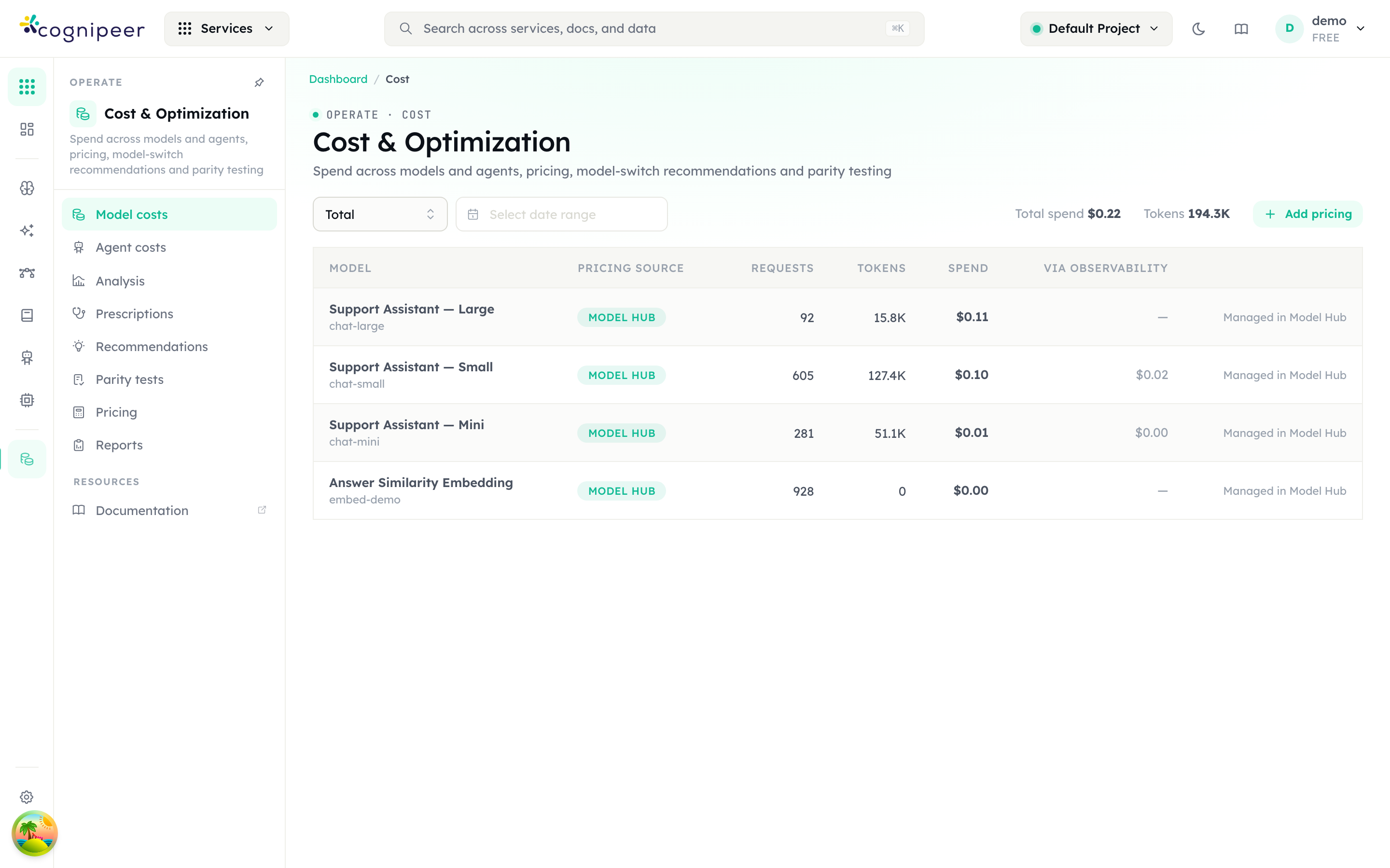
Model costs: the Pricing source column is the one to read first. Spend is only trustworthy for rows that are not Unpriced — an unpriced row contributes real tokens and $0 of spend. The via Observability column separates trace-derived spend from gateway traffic.
Rows arrive from two directions. Calls that went through the console gateway land with source api. Calls the agent made directly to a provider land with source tracing, ingested from the agent's traces — which is why an agent that never touches the gateway still shows up here, as long as it reports traces (see Agent Tracing). The per-model split is carried on costBySource, and the Model costs table surfaces the trace-derived share in its via Observability column.
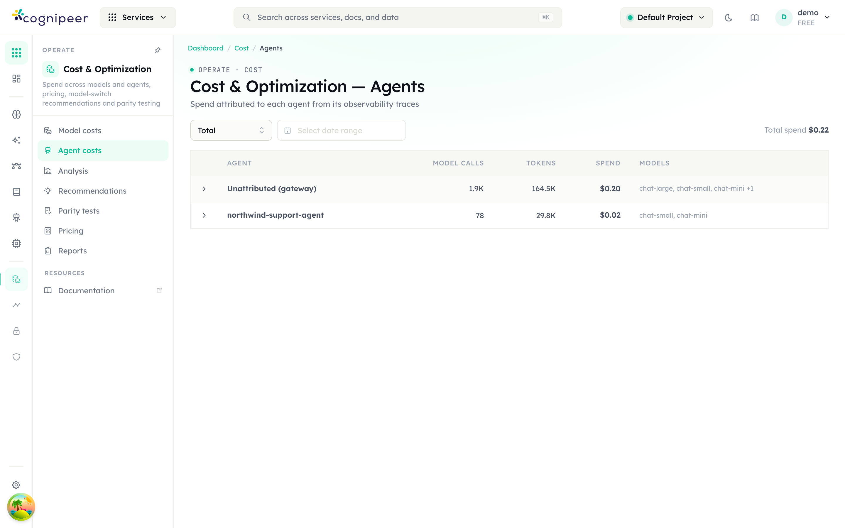
Agent costs groups the same rows by the tracing agentKey instead of the model, with a per-model composition inside each agent. Traffic with no agent attribution — plain gateway calls — is grouped under Unattributed (gateway). An agent whose models include an unpriced one is flagged: its spend reads low.
When any observed model has no price, both pages raise a banner. Model costs names how many models have usage but no pricing and how many tokens were recorded at $0; Agent costs names how many agents use models without pricing and links to the Pricing page.
Pricing
Pricing is the full catalog: every Model Hub model in scope, every external pricing entry, and every model observed in usage in the range — merged case-insensitively. Prices are effective-dated: an entry holds a list of versions, and the price used for a given UTC day is the version with the latest effectiveFrom on or before that day.
The Add pricing form takes the model name exactly as it appears in trace events (case-insensitive), the three rates — Input tokens — USD per 1M, Output tokens — USD per 1M, Cached input tokens — USD per 1M (optional) — and an Effective from day. Model Hub keys are rejected here on purpose: hub pricing always wins for hub models, so a catalog entry for one would be dead weight. When observed models are unpriced, Match from catalog bulk-matches them against the public market price feed.
Entering a price prices ingests from then on
This is the single most common surprise in the whole service. Cost is computed at ingest and written onto the rollup row. Entering a price today does not retro-price yesterday's traffic — recorded history is never rewritten by an edit. A model that ran for a month unpriced keeps a month of $0 rows.
The escape hatch is deliberate and manual: the Recalculate action on an external entry (POST /api/cost/pricing/reprice) walks the recorded rows and recomputes each one with the price effective on that row's day. The pricing form carries the same thing as a Recalculate recorded spend switch. Rows whose day is covered by no version keep their existing cost — an unknown price is not a free price. Model Hub models are rejected: their history was computed from hub pricing at ingest and is not repriceable here.
The external market price feed has its own endpoints (/api/model-price-catalog*): status, a paged entry listing, per-name suggestions, and a manual refresh. There are no background timers or schedulers — the in-memory catalog is refetched lazily when it is empty or older than 24 hours, and the refresh endpoint forces one.
Analysis
Analysis (/dashboard/cost/analysis) is the deterministic metric surface: "Deterministic, reproducible metrics from live traces — analyse an agent or a model, then jump into optimization". A segmented control switches between Agents and Models; window tiles show Sessions, Total tokens, Cache hit and Output share.
Underneath sit the cards that Prescriptions later reads as evidence: Deterministic insights (Tool menu / call, Tool schema complexity, Traffic language, AI calls / session, Tool calls / session, Input tokens / AI call, System prompt), System prompt checks, Repeated tool calls and Recurring errors. In model mode there is also Agents using this model. The header links out to Full observability (agent mode only) and Run model matrix.
The eight prompt checks — Size budget, Duplicate paragraphs, Duplicate sentences, Overall repetitiveness, Dynamic content in prefix (cache killer), Placeholder / unfinished content, Whitespace hygiene, Invisible / control characters — each report PASS, WARN or FAIL.
Rather than repeat the walkthrough here: Optimize token usage takes an agent from instrumentation through analysis, snapshot, evaluation and proof in one pass. Read that first if you are working an agent end to end.
Prescriptions
Analysis shows you numbers. Prescriptions decides which of those numbers are problems.
Automated analysis over observed traffic: deterministic detectors turn tracing + cost evidence into findings with prescribed actions. Numbers come from detectors only — nothing is estimated by a model.
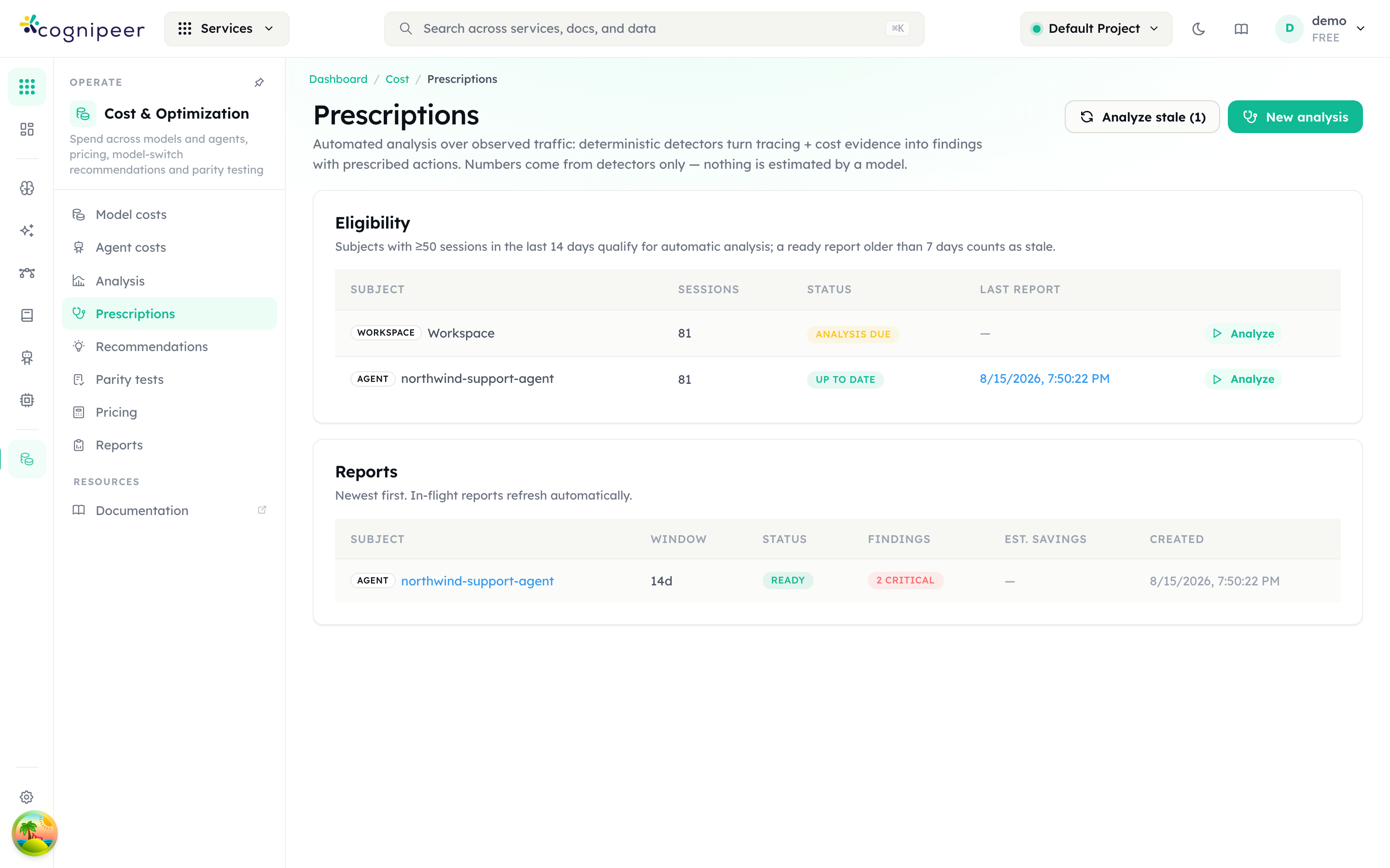
The list is two cards. Eligibility is the trigger surface — it states the thresholds in words and marks each subject analysis due, up to date or not enough data. Reports is the history, newest first; the Findings column summarises severity counts and Est. savings shows — where nothing could be priced.
What a report is
A report is generated for one subject over one window:
| Subject kind | Evidence used |
|---|---|
| Agent | The agent's tracing overview + its cost entry |
| Model | The model's tracing overview + its observed-cost entry |
| Workspace (all traffic) | The workspace cost report + per-agent costs + every observed model |
The New analysis overlay collects the subject (section Subject: Kind, then Agent or Model name) and the window (section Window: Analysis window — Last 7 days, Last 14 days or Last 30 days), then Run analysis. Generation is asynchronous: evidence gathering reads full session windows, so it never runs inside the HTTP request. The report row appears immediately as pending, moves to running, then to ready or failed, and the page polls on its own.
While a report for the same subject is pending or running, asking for another one returns the in-flight report instead of enqueueing a duplicate.
Eligibility and the auto-run
The Eligibility card renders the rule with the live values substituted: Subjects with ≥N sessions in the last W days qualify for automatic analysis; a ready report older than S days counts as stale.
| Threshold | Environment variable | Default |
|---|---|---|
| Sessions needed in the window | PRESCRIPTIONS_MIN_SESSIONS | 50 |
| Age at which a ready report is stale | PRESCRIPTIONS_STALE_DAYS | 7 |
The header's Analyze stale (N) button runs every eligible subject whose latest ready report is stale. It is scoped to the current tenant only, and it enqueues the workspace report plus at most ten agents per call. A subject with an in-flight report is never counted stale, so repeated clicks cannot pile up duplicates.
Eligibility lists the workspace and the agents observed in the window. Model subjects are not listed there — request one from New analysis with kind Model.
Finding anatomy
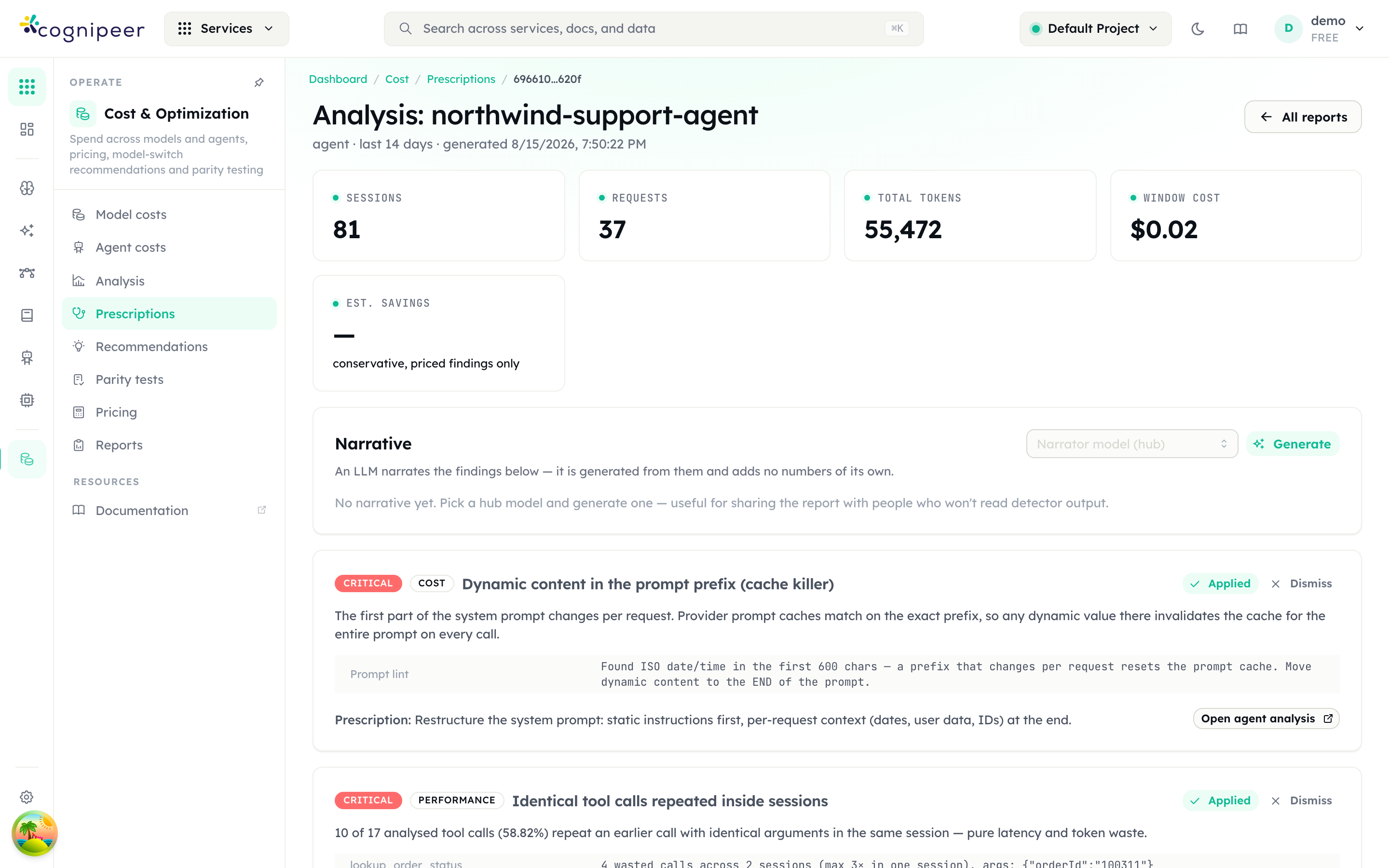
A report with two critical findings. Read a card top-down: severity badge, category badge, title; the summary states what was measured; the evidence table shows the measured values the detector used; the bold Prescription: line is the action; the CTA on the right jumps to the screen where you fix it. Note the Est. savings tile reading — — no finding in this report could be priced, and the tile refuses to invent a number.
Every finding carries:
| Part | Values / notes |
|---|---|
| Severity | critical, warn, info — findings are ordered by severity, then by savings |
| Category | cost, reliability, performance, hygiene |
| Summary | States the measurement, and the threshold that fired where the detector has one |
| Evidence | Label/value rows taken verbatim from the measured data |
| Prescription | The concrete action, plus an optional CTA |
| Est. savings | A conservative monthly estimate, or null |
The CTAs are the ones the detectors emit: Open agent analysis, Open agent sessions, Open pricing, Open cost by agent, Open recommendations.
null savings means unpriceable, not zero
estMonthlySavingsUsd is null whenever the problem is real but cannot be priced from available data — typically because the model has no price, or no cached-token rate is known for it. The estimate is never guessed to fill the column. Cache savings, for example, are only computed when the model's pricing has both an input rate and a cached rate, and they are scaled to a conservative 50% attainable cache rate. Everything else reports —.
Lifecycle
Each finding has an action pair: Applied and Dismiss, with Reopen on a dismissed one. applied is what makes the loop closable — mark the fix, re-run the report on the same subject later, and the detector either goes quiet or does not. Dismissed findings stay on the report, dimmed.
The narrative
The detail page has a Narrative card — "An LLM narrates the findings below — it is generated from them and adds no numbers of its own." Pick a hub model in the Narrator model (hub) select and press Generate (Regenerate afterwards).
Its role is strictly bounded, in the prompt and by design: it receives the finished findings as JSON and may use only figures that appear there, verbatim. It may not add findings, causes or savings; a finding with null savings gets no dollar figure attached. It orders by severity and writes a short executive summary. It runs only against a ready report. If you want to know where a number came from, the answer is always a detector — never the narrator.
The 17 detectors
The detector battery is the whole engine. Each detector runs only for the subject kinds it applies to, and a detector that throws is skipped rather than sinking the report.
Cost
| Finding | Subjects | Fires when |
|---|---|---|
| Prompt cache barely used | agent, model | Cache hit rate below 40% over ≥1M input tokens in the window; critical below 10%. Names the dynamic-prefix lint check as the likely cause when that check is not passing |
| Dynamic content in the prompt prefix (cache killer) | agent, model | The dynamic-prefix prompt-lint check is not passing; FAIL → critical |
| System prompt over the size budget | agent, model | The size prompt-lint check is not passing; reports estimated tokens and characters |
| Very large context per model call | agent, model | Average input tokens per AI call ≥20,000; critical at ≥50,000 |
| Tool menu larger than the agent uses | agent, model | Average menu ≥30 tools per call, or ≥10 offered tools were never called in the window |
| Anomalous spend days | workspace | Daily spend days that sit far outside the workspace's own baseline (robust z ≥ 5) |
| Spend has shifted to a higher level | workspace | The last 7 days' median daily spend is at least 2× the prior two weeks' median. A drop by the same factor is reported as info under the mirrored title |
| Spend concentrated on premium-tier models | workspace | ≥70% of priced spend on top-tier models, with ≥$50 total priced spend. Severity info — it is a candidate for testing, not a defect |
| Models with heavy input volume and low cache hit | workspace | Models with ≥1M input tokens and a cache hit rate below 40%, ranked by priced opportunity |
Reliability
| Finding | Subjects | Fires when |
|---|---|---|
| The same error keeps recurring | agent, model | One error signature occurred ≥10 times in the window; critical at ≥50 |
| Elevated session error rate | agent, model | ≥5% of sessions ended in error, over at least 20 sessions; critical at ≥15% |
| Tools failing at a high rate | agent, model | A tool with ≥20 calls and an error rate ≥30%; critical when any reaches 70% |
| High request error rate across the workspace | workspace | ≥5% of at least 100 model requests errored; critical at ≥15% |
Performance
| Finding | Subjects | Fires when |
|---|---|---|
| Identical tool calls repeated inside sessions | agent, model | ≥10 wasted calls and ≥10% of analysed tool calls repeat an earlier call with identical arguments in the same session; critical at ≥30% |
Hygiene
| Finding | Subjects | Fires when |
|---|---|---|
| Abnormal traffic spike days | agent, model | Daily session counts deviate massively from the subject's own baseline (robust z ≥ 6) |
| Token usage with no price attached | workspace | Any tokens recorded against unpriced models; critical when ≥20% of the window's tokens |
| Same model recorded under multiple keys | workspace | Two or more usage keys normalize to the same underlying model name |
API
Eight session-authenticated dashboard routes:
| Method | Endpoint | Description |
|---|---|---|
GET | /api/prescriptions | List reports (project-scoped) |
POST | /api/prescriptions | Enqueue a report → 202 |
POST | /api/prescriptions/auto-run | Enqueue for every stale eligible subject → 202 |
GET | /api/prescriptions/eligibility | Which subjects qualify, and which reports are stale |
GET | /api/prescriptions/:id | Report detail (the UI polls this) |
DELETE | /api/prescriptions/:id | Delete a report |
PATCH | /api/prescriptions/:id/findings/:findingId | Finding status: open / applied / dismissed |
POST | /api/prescriptions/:id/narrative | Generate the narrative over a ready report |
The window defaults to 14 days and is clamped to 3–90 days server-side, whatever the UI offers. See the Cost & Prescriptions API.
Recommendations
Enterprise module
Recommendations is part of the enterprise edition. The /api/abacus/* routes behind it are licence-gated per tenant and answer 402 without one. See Licensing.
/dashboard/cost/recommendations — "Optimization opportunities computed from observed usage — cost via pricing, latency via observed averages (no pricing needed)". (/dashboard/abacus is kept as an alias, so old links still resolve.)
Everything is computed on demand from the same usage_daily rollup, Model Hub pricing and the external pricing catalog. Trace-derived rows participate automatically, so agents that call providers directly are covered as long as their traces land in the console.
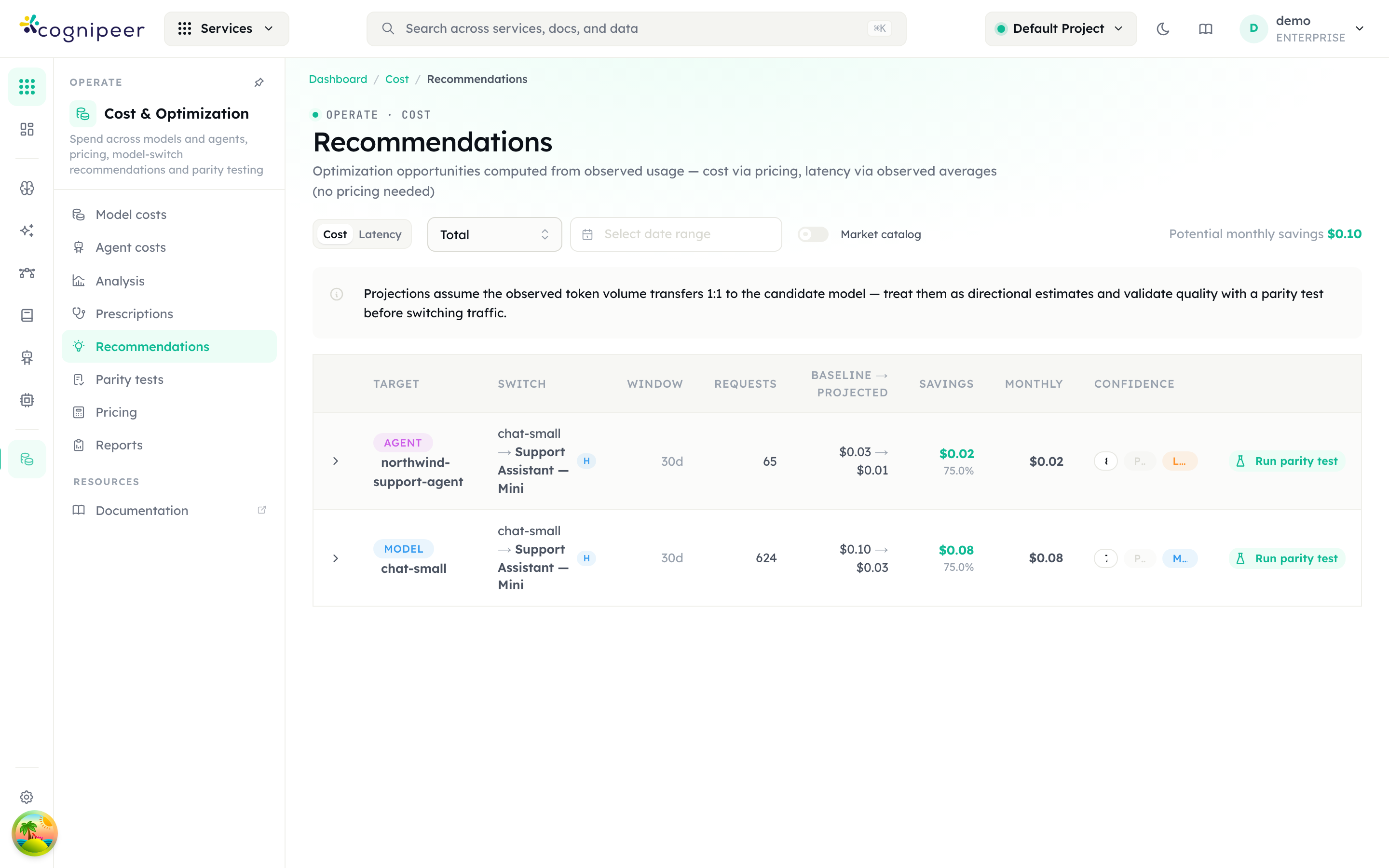
Two rows, one per target — an agent and a model — each proposing the same switch. The banner above the table is the important part: projections assume the observed token volume transfers 1:1 to the candidate, so they are directional until a parity test measures the real ratio.
Expanding a row is where the reasoning lives.
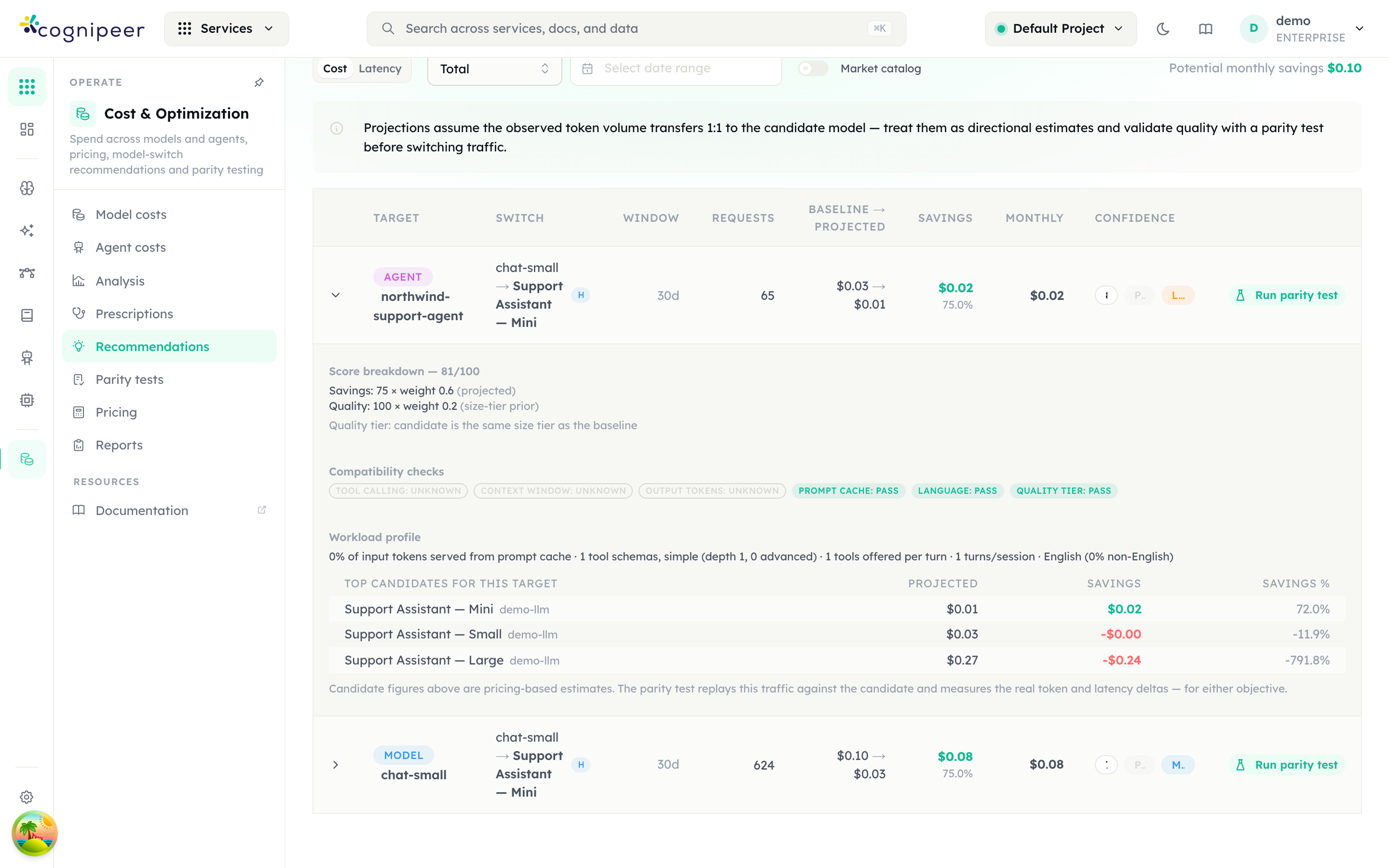
Note the Compatibility checks row: three gates read UNKNOWN and the candidate is still ranked. Unknown is not a failure — see Hard gates below. Workload profile summarises what the traffic actually looks like, and Top candidates for this target shows the alternatives that were considered, including ones that would cost more (a negative saving).
Objectives
A segmented control picks Cost or Latency.
| Objective | Ranks on | Needs |
|---|---|---|
| Cost | Projected spend if the observed token volume ran on the candidate | Priced usage |
| Latency | Observed average latency from the rollup's latency counters | Nothing but traffic — the on-prem path |
Default thresholds: a segment must clear 50 requests, and a candidate must beat the baseline by 20% (savings, or latency gain) to surface. Each is overridable per request (min_requests, min_savings_pct, min_latency_gain_pct).
The Market catalog switch
Candidates come in three tiers, and the tier decides how actionable the advice is.
| Tier badge | Source | Actionability |
|---|---|---|
| Hub | A Model Hub LLM | Routable and parity-testable |
| External | Observed in the window, priced by the external catalog | Advice — the console cannot route to it |
| Market | The community market price feed | Advice — add it to the hub to make it actionable |
The Market catalog switch appears under the Cost objective only, and it is off by default. While it is off the market tier is not considered at all — only hub models and externally-priced observed models are, so an empty or dull feed is very often this switch alone. That is also where the open-weight universe lives: with the switch off, the only open-weight candidates you can see are the ones already in your Model Hub. Turning it on widens the pool to the whole priced, chat-capable market, deduplicated across hosts so a top-N cut is not filled with N copies of one model.
Columns
The shared columns are the expand caret, Target, Switch, Window, Requests, the objective-specific block, Confidence, and the row action. The objective changes the middle:
| Objective | Extra columns |
|---|---|
| Cost | Baseline → projected · Savings · Monthly |
| Latency | Tokens/req · Avg latency · Gain |
Row badges carry the rest: the tier (Hub / External / Market), Open weights, No cache rate (the candidate publishes no prompt-cache price, so the cached slice of the prompt was projected at its full input rate — the saving shown is real but conservative), the evidence tier (Projected / Compatible / Parity-proven) and confidence (High confidence / Medium confidence / Low confidence, driven by traffic volume).
The expanded row
Expanding a row opens five blocks:
| Block | What it shows |
|---|---|
| Score breakdown | The weighted components behind the composite score — savings, latency, quality — each labelled with its source (projected, measured, parity evidence, or size-tier prior) |
| Compatibility checks | Each gate that ran, with pass or unknown, plus the count excluded by failed gates |
| Workload profile | Cache rate, tool schema count/band/depth, tools offered per turn, turns per session, primary language and non-English share |
| Self-hosting | For open-weight candidates: GPUs required, $/hour, $/month, expected tok/s, and break-even versus observed utilisation |
| Parity evidence | The matched parity run: pass rate, average score, items, measured token ratio and latency, with a link to the run |
Hard gates, and why unknown never excludes
Seven deterministic gates run before ranking. Capability facts come from the market price catalog, where an absent fact means unknown, never false.
| Check id | UI label | Excludes a candidate when |
|---|---|---|
tools | Tool calling | The workload calls tools and the candidate is known not to support them |
contextWindow | Context window | The candidate's known max input is smaller than the observed requirement |
outputTokens | Output tokens | The candidate's known max output is smaller than the observed requirement |
qualityTier | Quality tier | The candidate is more than one size tier below the baseline |
promptCache | Prompt cache | ≥40% of the segment's input comes from cache and the candidate publishes no cache price |
toolComplexity | Tool complexity | The candidate is below the tier floor the workload's tool schemas, menu size and turn horizon demand |
language | Language | At least 50% of the classified traffic is non-English and the candidate is documented English-first |
Two rules matter more than the list:
A candidate that fails a gate is not shown at all. It is removed from the ranking and counted in the line "N candidates excluded by failed hard gates". A short candidate list on a cache-heavy, non-English, complex-tool workload is a finding, not a bug — the Workload profile block exists to show you why.
Unknown never excludes. Only a known incompatibility removes a candidate. A gate with missing data records unknown, the candidate stays in the ranking, and — absent parity evidence — the row's evidence tier is held at Projected: the recommendation is still made, but not claimed as verified.
Parity evidence overrides the prompt-cache, language, quality-tier and tool-complexity gates for the exact pair it proves. Evidence beats prior, always.
Parity tests and Model matrix
Enterprise module
Parity tests and the model matrix are part of the enterprise edition, on the same licence-gated /api/abacus/* surface as Recommendations.
/dashboard/cost/parity — "Quality-parity runs launched from cost recommendations — snapshot, suite and evaluation run per test". (/dashboard/abacus/parity is an alias.)
Where a run starts
Not on this page. A parity run starts from the row action on Recommendations, which opens the Run parity test overlay with the subtitle <current model> → <candidate model>. The overlay collects:
| Field | Notes |
|---|---|
| Data source | Sample fresh traffic (mode snapshot) or Use existing dataset (mode existing-dataset) |
| Candidate model | A Model Hub LLM — the model under test. Pricing is not required |
| Judge model | A Model Hub LLM that scores answer equivalence against the recorded production answer |
| Evaluation dataset | Existing-dataset mode only — an imported, snapshot or hand-built dataset, already anonymized at creation |
| Sampling % / Max items | Snapshot mode only: defaults 10 and 100 |
| PII categories | Snapshot mode only — the anonymization gate is mandatory |
A market or external candidate cannot be replayed; add it to the Model Hub first.
In snapshot mode the run is three stages behind one button: sample the target's real traffic into an evaluation dataset (behind the PII gate), create a suite targeting the candidate with a tool-call scorer and an llm-judge scorer, and enqueue the run. Existing-dataset mode skips straight to the suite. The overlay reports progress as Parity test in progress → Evaluation run started, or Parity test failed. Nothing is cleaned up silently: if a later stage fails, the ids of the stages that succeeded are still linked, so a dataset created before a suite failure is inspectable.
The list on the Parity tests page has columns Created, Target, Switch, Judge, Items, Status and Links. The status badge reads Queued, Running, Ready or Failed (the underlying values are pending, running, ready, failed); a running row also names its stage. Results land on the normal evaluation run pages — see Evaluation & Analysis.
Model matrix
The Model matrix is a panel at the top of the Parity tests page, not a route of its own — the Run model matrix action on Analysis navigates here.
Replay ONE evaluation dataset against MANY candidate models and compare them side by side — pass rate, judge score, tool fidelity and measured cost per item.
Pick a Dataset, one or more Candidate models, a Judge model, and press Run matrix. Each candidate gets its own suite and run on the same dataset, enqueued in one launch and executed in the background; a candidate that fails validation is reported without stopping the others.
Results table: Candidate, Status, Pass, Judge, Tool fidelity, $ / item, Latency, Run. The Judge cell shows "N scored" under the average.
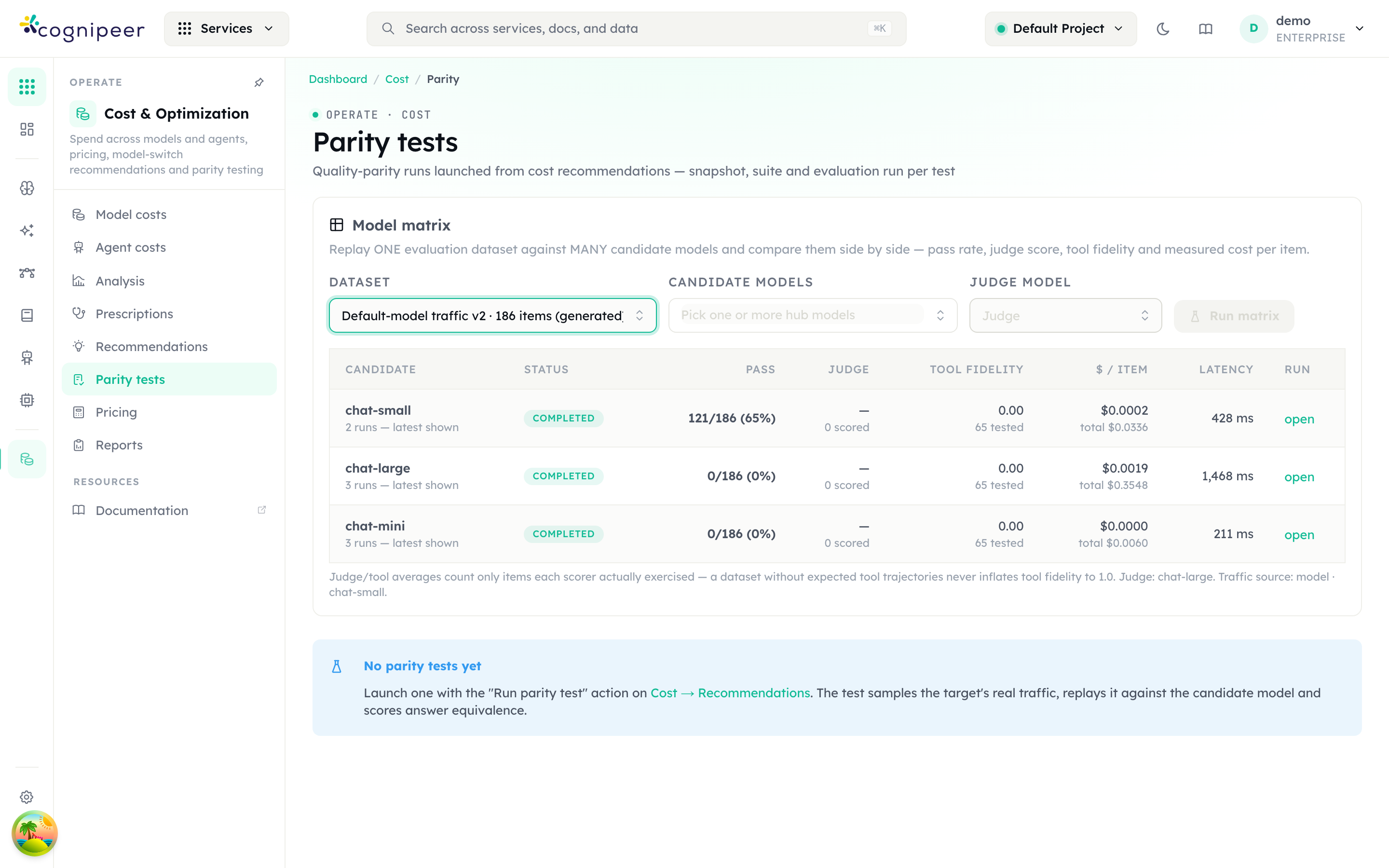
A run from the demo tenant, and a good example of why this exists. The recommendation engine had just proposed switching to the cheapest candidate on a projected 75% saving. The matrix replayed the same 186-item dataset against all three models and measured the incumbent at 65% pass while both alternatives scored 0% — the cheap model is not answering these questions the same way at all. A projection said switch; a measurement said no.
The footnote under the table matters too: judge and tool averages count only the items each scorer actually exercised. A dataset with no expected tool trajectories will show a tool fidelity of 0.00 over the items that were tested rather than a flattering 1.00 over none.
The judge cannot be trusted to grade itself
When the judge model is also among the candidates the panel says so:
Note: the judge model is also a candidate — its own row carries self-judgement bias.
Treat that row as indicative and confirm it with a different judge.
Two aggregation details keep the comparison honest. The tool-call scorer returns a perfect score when an item correctly expects no tools; averaging that blindly would inflate candidates on datasets without trajectories, so Tool fidelity averages only over items where tool behaviour was actually exercised (toolTested). Judge likewise averages only over items the judge actually scored (judgeScored) — which is what the "N scored" line reports. Neither average can be inflated by items that were never really tested.
What-if versus parity
These two words describe very different claims, and the difference decides how much you should trust a number.
| What-if (Recommendations) | Parity (Parity tests, Model matrix) | |
|---|---|---|
| Method | Static repricing of observed volume | A real replay of real traffic |
| Model called? | No | Yes — candidate and judge |
| Token volume | Assumed to transfer 1:1 to the candidate | Measured |
| Quality | A size-tier prior | Measured: pass rate, judge score, tool fidelity |
| Cost | Projected from published prices | Measured $ per item |
| Answers | "Which candidates are worth testing?" | "Did this candidate actually hold up?" |
What-if corrects itself. Once a completed parity run has measured a token ratio for a (current → candidate) pair, the recommendation engine stops using the 1:1 assumption for that pair and reprices with the measured ratio, marking the row as measured. The evidence tier reaches Parity-proven once that run is both large and clean enough — at least 50 completed items at a pass rate of 90% or better. The estimate is not a permanent guess; it is the starting point that evidence replaces.
There is deliberately no tokens objective. Under a 1:1 transfer assumption every candidate ties on tokens, so a static what-if cannot rank on it — the ranking would be meaningless rather than merely imprecise. Put plainly: cost needs pricing; latency works from observed averages and needs none; token savings cannot be estimated, only measured — which is exactly what a parity test is for.
Internal signals with no screen of their own
Three helpers produce numbers you will see attributed to other places:
| Helper | Where it surfaces |
|---|---|
| Workload signals | The Workload profile block on Recommendations (cache rate, tool schema band and depth, tool menu size, turns per session, primary language and non-English share), and the Tool schema complexity / Traffic language tiles on Analysis |
| Model traits | Not shown directly — it feeds the Quality tier row and the tier gate |
| GPU hourly rates | The Self-hosting block on Recommendations |
Self-hosting figures are indicative, not a quote
The $/GPU-hour numbers behind the Self-hosting block are order-of-magnitude public on-demand rates. They are not a quote: reserved capacity, spot and owned hardware all land well below them, so the estimate is conservative in the direction of "self-hosting looks more expensive". Override the rate per request with the gpu_hourly_usd query parameter.
Read the source field before quoting the block. fleet means it was sized on an accelerator the tenant actually owns; reference means there was no readable fleet and an H100 PCIe stood in. A reference estimate answers "is this worth exploring", not "this is your bill". See GPU Fleet.
Snapshot dataset items also carry a lang:<iso> tag, so parity and matrix results can be read per language rather than as one blended number.
Reports
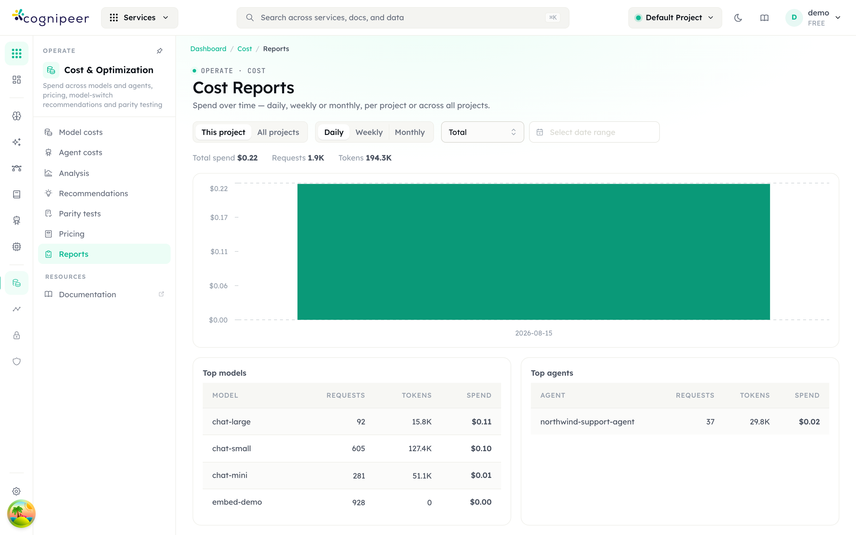
Cost Reports — "Spend over time — daily, weekly or monthly, per project or across all projects." Two segmented controls set the scope (This project / All projects) and the granularity (Daily / Weekly / Monthly), alongside a date filter.
The page shows the series table (Day / Week of / Month, Requests, Errors, Tokens, Spend) plus the top models and top agents for the range, each with Requests, Tokens and Spend. The same report is what the workspace-subject detectors read for spend anomalies, regime shifts and the workspace error rate.
For per-token, per-user and per-key attribution — budgets, quotas and spend grouping — see the Spend & Budgets API.
Things that surprise people
| Surprise | Why |
|---|---|
| Adding a price did not change last month's spend | Cost is computed at ingest and history is never rewritten. Use Recalculate on an external entry — hub models cannot be repriced |
| A model shows tokens but $0 spend | It is Unpriced. Add pricing, or use Match from catalog |
| An agent's spend reads low | One of its models is unpriced; the row is flagged for exactly this reason |
| A model appears twice under slightly different names | Split usage keys — the "Same model recorded under multiple keys" detector names them |
The savings column shows — | The finding is real but could not be priced. A number is never guessed to fill the column |
| Recommendations shows nothing useful | The Market catalog switch is off by default, and without it the whole market tier — and with it nearly every open-weight candidate — is never considered |
| A cheap model you expected is missing | It failed a hard gate and was excluded, counted in "N candidates excluded by failed hard gates". Unknown capability never excludes — only a known incompatibility does |
| Latency recommendations appear where cost ones do not | The latency objective needs no pricing at all; the cost objective cannot run on unpriced traffic |
| The narrative added no new insight | By design. It narrates the findings and is forbidden from introducing numbers, causes or savings of its own |
| Prescriptions ignores a busy agent | It is below PRESCRIPTIONS_MIN_SESSIONS in the window, or a report already exists and is not yet stale |
| The judge model scored itself well | If it is also a candidate, the panel warns about self-judgement bias — re-run with a different judge |
| Enterprise pages return 402 | Recommendations, Parity tests and the model matrix are enterprise; every /api/abacus/* route is licence-gated per tenant |
Step by step: optimize token usage
This is the long one. It takes an agent you already run in production and walks the whole loop: connect it, measure it, sample its real traffic into a dataset that is safe to keep, build a test you can re-run, compare models honestly, cut tokens, and prove the cut did not cost you quality.
Nothing here requires rewriting your agent. The framework stays exactly as it is.
Who this is for
Both halves of the team. The click-paths are written so an operations lead can follow them without touching code; each section then gives the engineer the endpoint, the payload and the trap.
What you end up with
your agent ──► traces ──► insights ──► traffic snapshot ──► dataset
                                                              │
                            ┌─────────────────────────────────┘
                            ▼
                     evaluation suite ──► baseline run
                            │
                            ├──► same suite, different model   → is the cheap one good enough?
└──► same suite, after your change → did the change break anything?Be clear-eyed about the scope. This measures and reduces your token usage: the prompt you send, the tool menu you attach, the calls your loop makes. It does not change what your framework sends on your behalf, and it is not a magic compression layer.
Before you start
| You need | Where |
|---|---|
| An API token with tracing enabled | Settings → API Tokens → Create Token |
| At least one model in the Model Hub | See Create your first model |
| Pricing filled in on that model | Model Hub → the model → pricing fields |
| An agent that already runs | Any framework — LangChain, LangGraph, OpenAI Agents, your own loop |
Fill in pricing first
A model with zero pricing reports zero spend forever, and every cost number in this guide stays blank. Pricing is applied at ingest time and history is never rewritten, so a price entered today does not retro-price yesterday's traffic. Set it before you start collecting.
Act 1 — Connect the agent you already have
Two lines of setup. No proxy, no base-URL swap in your agent, no code restructuring.
import cognipeer_observability as cognipeer
from cognipeer_observability.langchain import CognipeerCallbackHandler

cognipeer.init(agent={"name": "support-agent"})

result = agent.invoke(
    {"input": question},
    config={"callbacks": [CognipeerCallbackHandler(thread_id="conv-42")]},
)COGNIPEER_API_KEY=cpeer_…
COGNIPEER_BASE_URL=https://your-console-host # host root, no /api/client/v1
COGNIPEER_CAPTURE_CONTENT=all # all | metadata | noneSet COGNIPEER_CAPTURE_CONTENT=all for this exercise. You are going to build a dataset out of these traces, and that needs the message bodies. metadata keeps structure and token counts but drops content, which is the right setting for steady-state operation once you have your dataset.
Full SDK reference, and the wiring for LangGraph, OpenAI Agents, Claude Agent SDK, Vercel AI SDK, n8n and plain OpenTelemetry, lives in Observability Integrations. If your framework is not covered, post sessions straight to the ingest endpoint — see Trace an existing agent.
Get the event types right, or half this guide goes blank
The deterministic insights in Act 3 key off canonical event types. A model call must be recorded as ai_call and a tool invocation as tool_call. Anything else still draws a perfectly readable timeline — and then Tool menu, AI calls per session, System prompt and Repeated tool calls all come back empty. The SDK does this for you. Hand-rolled ingest is where people get caught; the correct shape is in Trace an existing agent.
Act 2 — Watch it for a day
Let real traffic accumulate. You are looking for a representative window, not a big one.
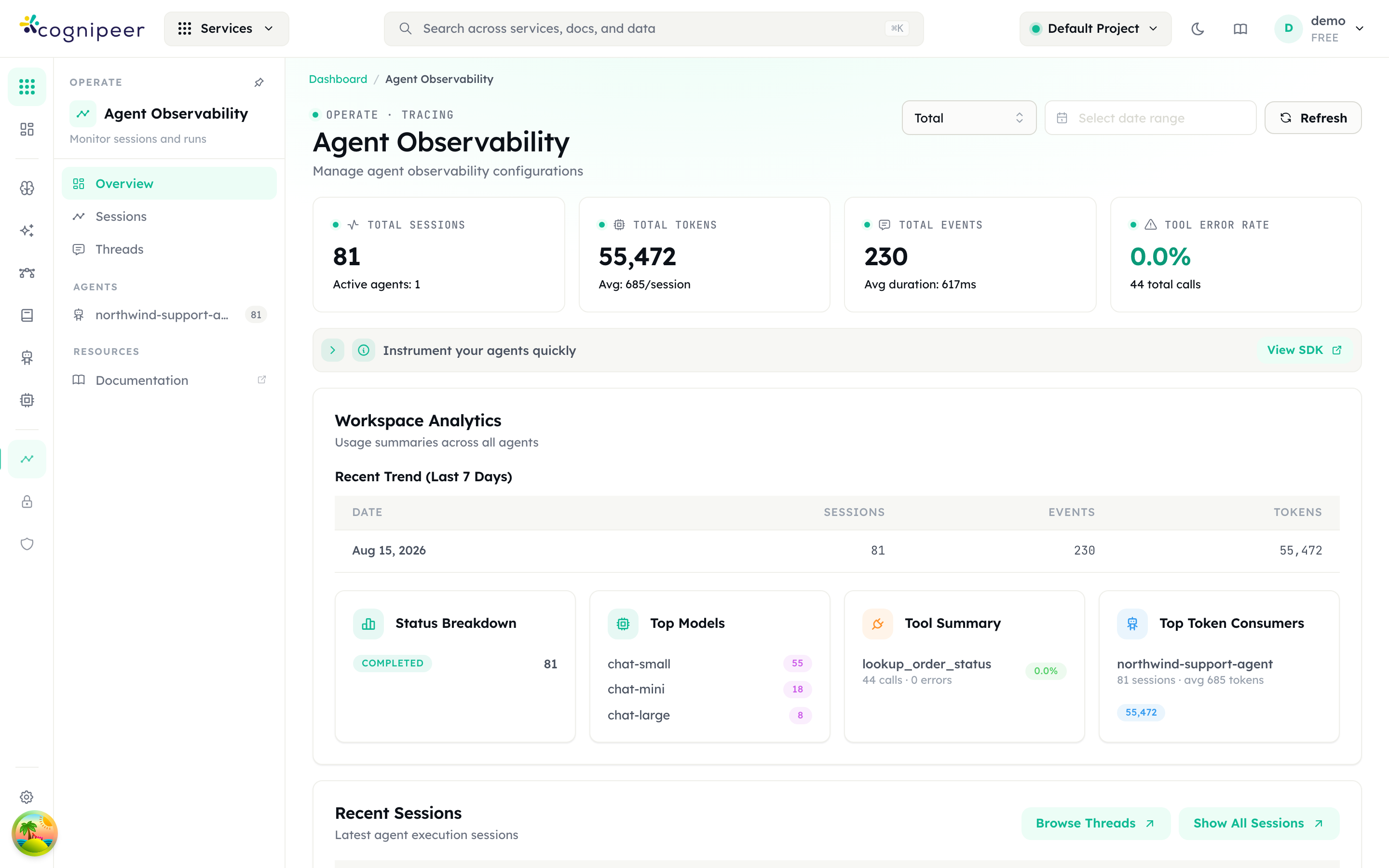
Go to Agent Observability.
Open a single session to see what one conversation actually cost.
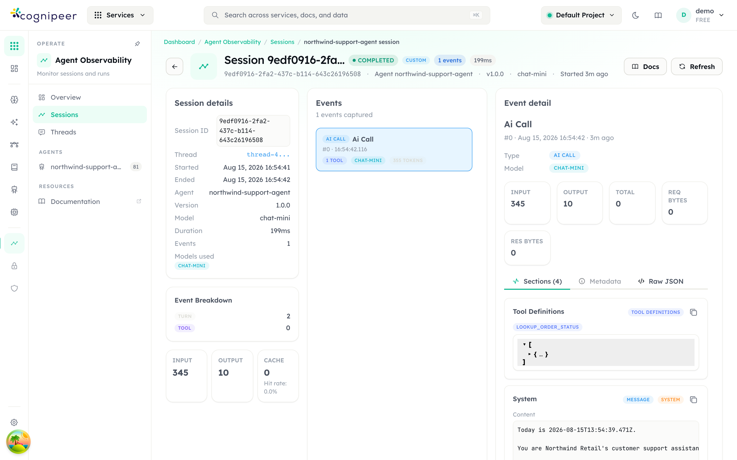
The thing to look at is the Tool Definitions card on each turn. That is the tool menu the model was sent on that call — and it is re-sent on every call. A ten-tool menu on a six-call session is that menu paid for six times.
Then switch to money: Cost & Optimization → Agent costs attributes spend to each agent from its traces, and Reports gives you the trend line you will compare against later.
Act 3 — Read the deterministic insights
Cost & Optimization → Analysis. Set the dimension toggle to Agents and pick your agent.
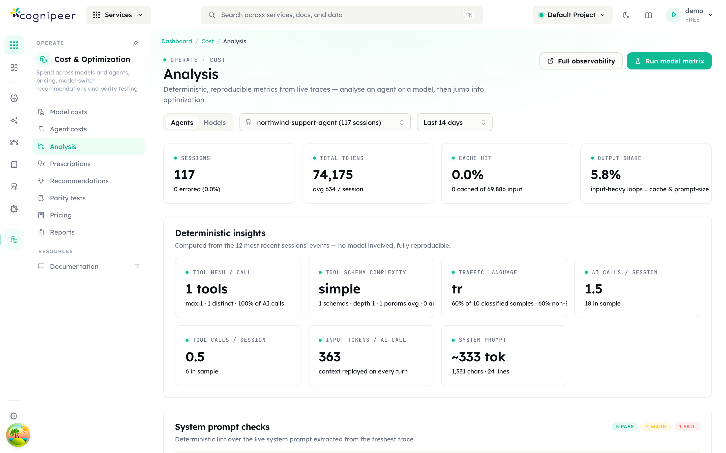
Everything on this screen is computed from raw trace events. No model is involved, so two people running it an hour apart get the same answer.
The demo tenant used for these screenshots shows:
| Insight | Value | What it means |
|---|---|---|
| Tool menu / call | 1 tool, 100% of AI calls | The menu is re-sent on every call |
| Tool schema complexity | simple — 1 schema, depth 1 | Fat, deeply nested tool schemas cost tokens on every call |
| Traffic language | tr — 60% of classified samples, 60% non-English | Which language your users actually write in |
| AI calls / session | 1.5 | Every extra call re-sends the whole context |
| Tool calls / session | 0.5 | More than one means loops — check the waste card |
| Input tokens / AI call | 363 | Context replayed on every turn |
| System prompt | ~333 tokens | Multiply by AI calls per session |
Read it as a hit list, in this order:
- Tool menu × AI calls per session is usually the single largest line item. It is also the easiest to cut, because most agents carry tools they never call. Tool schema complexity tells you whether the menu is expensive because it is long or because each entry is bloated.
- Repeated tool calls is free money — see below.
- System prompt is a fixed cost paid on every single call.
Traffic language is a model-choice input, not trivia
If most of your traffic is not English, a candidate model documented on English benchmarks is a risk you can measure rather than assume. The signal abstains rather than guessing — samples shorter than about eight words come back undetermined, and unclassifiable samples are excluded from the shares instead of being counted as English. A tenant serving Turkish support sees tr, not a confident en.
System prompt checks
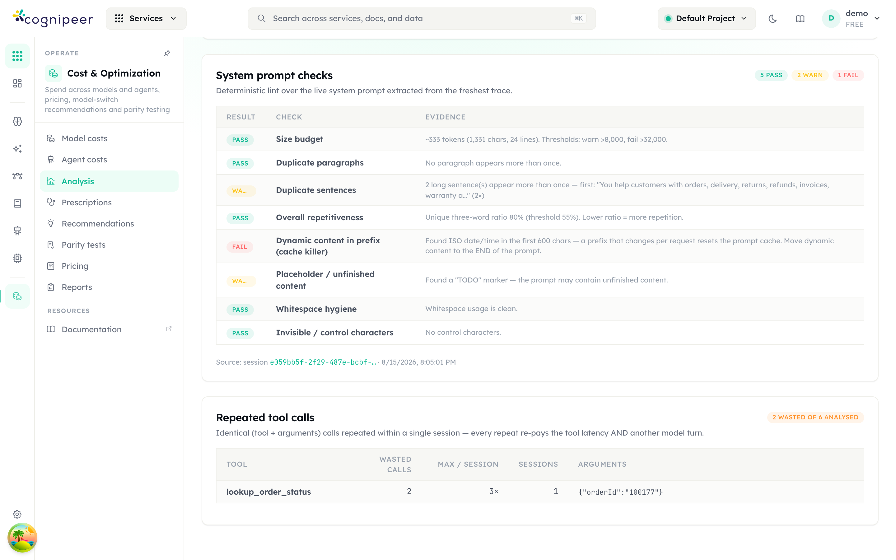
The System prompt checks card runs deterministic lint rules against the live prompt pulled from your traces. On the demo agent it returns 5 pass, 2 warn and 1 fail:
| Result | Check | Evidence |
|---|---|---|
| FAIL | Dynamic content in prefix (cache killer) | ISO date/time found in the first 600 characters |
| WARN | Duplicate sentences | 2 long sentences appear more than once |
| WARN | Placeholder / unfinished content | A TODO marker is still in the prompt |
The failure is the expensive one and it is extremely common. The demo prompt opens with Today is 2026-08-15T…. A prefix that changes on every request invalidates the provider's prompt cache every single time, so you pay full input price on every call forever. Move dynamic content to the end of the prompt. That one edit is often the largest single saving available, and it costs nothing.
Repeated tool calls
Identical calls — same tool, same arguments, same session. Every repeat pays the tool's latency and another model turn to process a result the agent already had.
In the demo sample the badge reads 2 wasted of 6 analysed — one order was looked up three times in a single session. The table names the tool, the exact arguments, how many sessions are affected and the worst case, which is usually enough to find the bug without opening a single trace. This is almost always a fault in how tool results are fed back into the loop, not a model problem.
The card reads the most recent sessions only, so the ratio moves as traffic does. Treat it as a signal to act on, not a metric to track.
Act 3b — Or have the detectors read it for you
Act 3 is the manual read. Cost & Optimization → Prescriptions runs the same kind of analysis automatically: a battery of deterministic detectors over the window's tracing and cost evidence, each one producing a finding with its evidence and a prescribed action.
Pick a subject — one agent, one model, or the whole workspace — and a window, then Run analysis.
The report above is the demo agent from this guide, generated at a point in time — a report is a stored snapshot of its window, which is why its numbers do not move with later traffic the way the Analysis cards do. The detectors independently found the same two problems Act 3 found by hand:
- Dynamic content in the prompt prefix (cache killer) — critical, cost
- Identical tool calls repeated inside sessions — critical, performance, "10 of 17 analysed tool calls (58.82%) repeat an earlier call with identical arguments in the same session"
Each finding carries its evidence, a Prescription: line naming the fix, and a conservative monthly savings estimate. Findings track as Applied / Dismiss / Reopen, so a report doubles as a worklist.
Two properties worth knowing:
- A savings figure is never guessed. When a problem is real but cannot be priced — an unpriced model, say — the estimate is left blank rather than invented. A dash there means "we will not put a number on this", not "this is free".
- The narrative does not do the analysis. The optional Generate button has a model write prose from the findings; it adds no numbers of its own. Useful for sharing a report with people who will not read detector output.
Prescriptions is the faster path. Act 3 is still worth doing once, because it teaches you what the detectors are looking at.
Act 4 — Turn real traffic into a dataset you are allowed to keep
You cannot compare models on invented questions. You need the questions your users actually ask — and you need them without the personal data attached.
Evaluations → Create from traffic, or Agent Observability → Create snapshot from traffic.
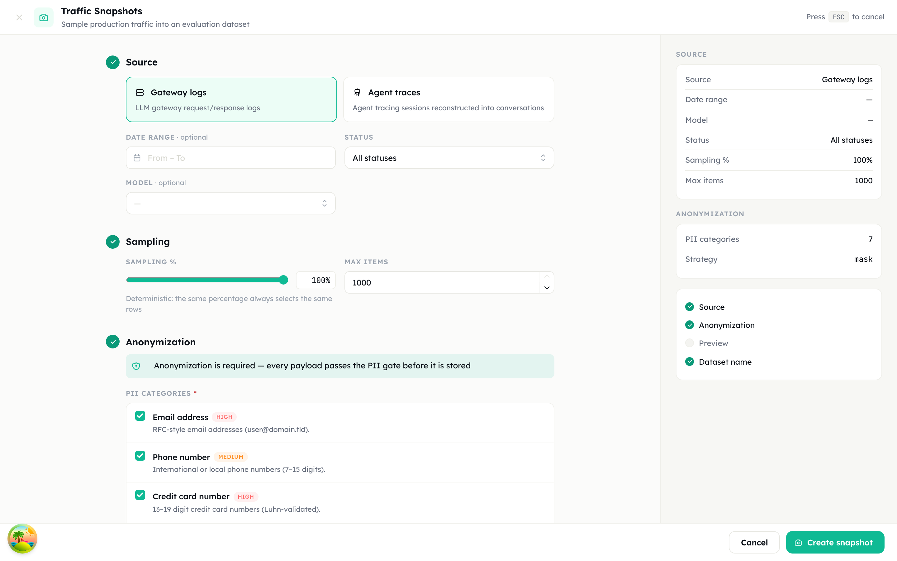
Four sections:
1. Source. Gateway logs (LLM gateway request/response logs) or Agent traces (tracing sessions reconstructed into conversations). Filter by date range, status, and — importantly — by Model.
Filter to one model
If you are deciding whether to replace model X, snapshot X's traffic. A snapshot spanning three models gives you reference answers from three different models, and then nothing you measure means anything.
2. Sampling. Sampling % is deterministic: the same percentage always selects the same rows, so a re-run of the snapshot is reproducible. Max items caps the result.
3. Anonymization. Not optional — "Anonymization is required — every payload passes the PII gate before it is stored". Creation is rejected outright without it. Pick your PII categories, then a Strategy:
| Strategy | Output | Use when |
|---|---|---|
| Mask | j***@domain.com | You only need the shape of the data |
| Pseudonym | <EMAIL_a1b2c3> | You are going to evaluate on it |
Prefer Pseudonym here. The token is HMAC-SHA256(salt, value), so the same person is the same token everywhere in the conversation — "email <EMAIL_a1b2c3> … reply to <EMAIL_a1b2c3>" still reads as one coherent exchange, which is what makes the dataset evaluable. The original value cannot be recovered without the salt, and the salt is never stored. Supply your own Stable salt if you want tokens to line up across several snapshots; leave it blank and the server generates a throwaway one for that run.
4. Preview. Run it before creating. You get Matching, Would sample, Would create and Scanned, plus a per-model breakdown.
The demo snapshot: 518 matching gateway rows for chat-small, sampled at 40% → 186 items created, 0 skipped, 85 PII findings replaced.
Read the skipped counters
"Not reconstructable" and "Payload budget reached" are not cosmetic. They mean your dataset is a biased subset of your traffic. Report them alongside any result you publish.
Act 5 — Make it repeatable, and establish a baseline
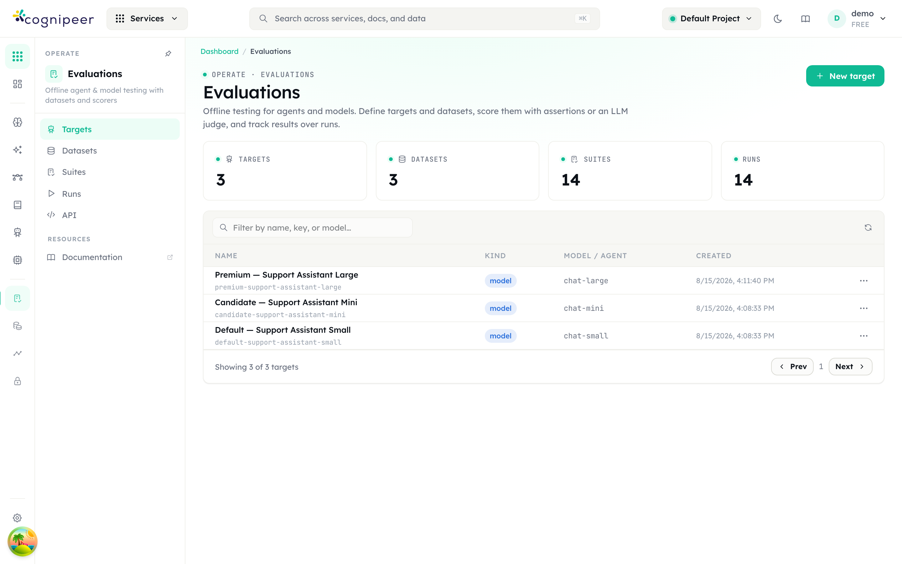
Evaluations → New target (Kind = Model, pick the model) → New suite (target + the snapshot dataset + scorers) → run it.
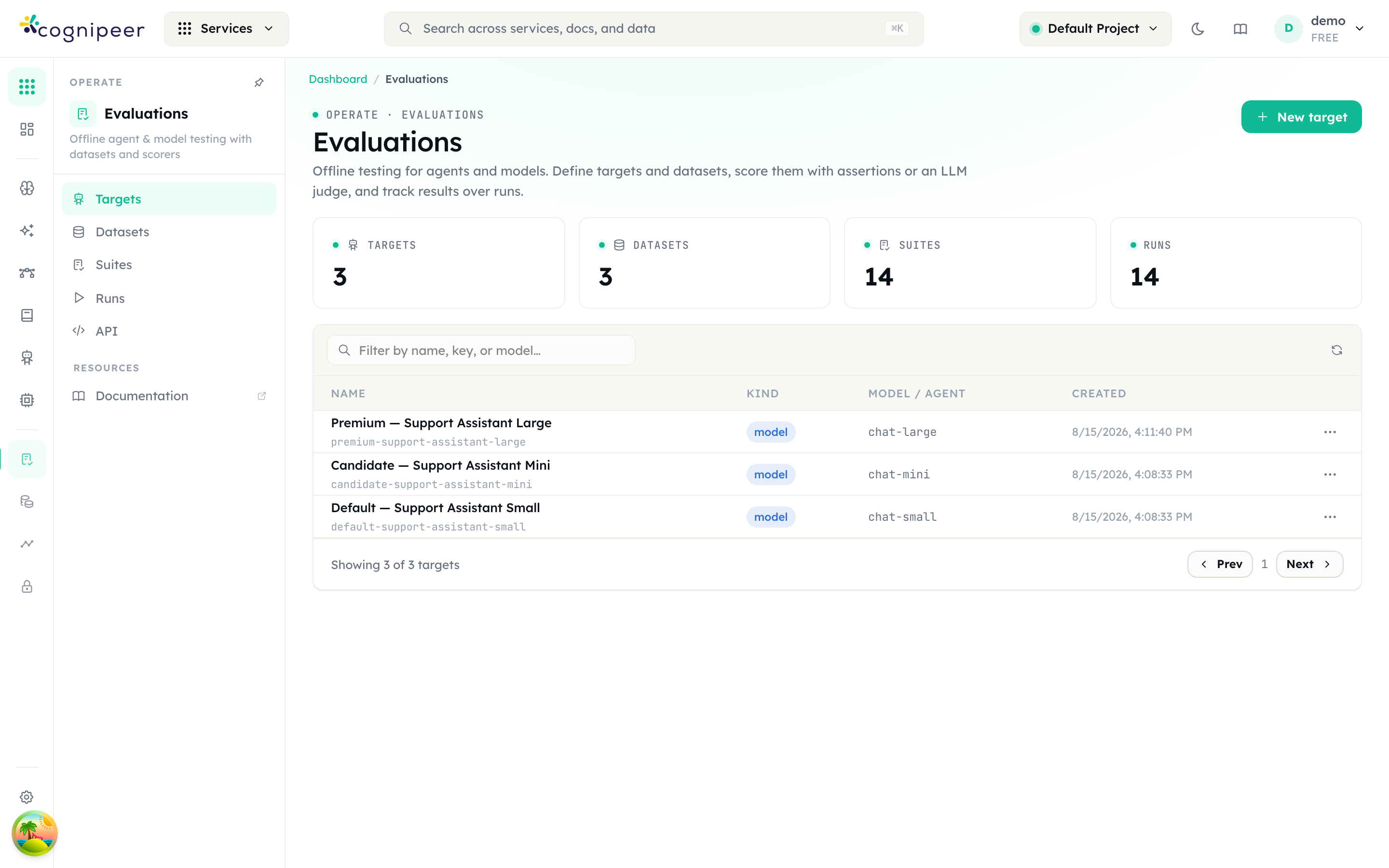
Run the incumbent model against its own recorded answers first. This is your control, and it is the step people skip.
Your control run tells you how much of your dataset is actually measurable
On the demo dataset the control scored 0.602. That is not a quality problem — 112 of the 186 items carry a reference answer, and the control passed every single one of them. 112 / 186 = 0.602.
The other 74 items are turns where production answered with a tool call, not text. They have no reference answer, so a similarity scorer scores them zero no matter which model you run.
If you had not run the control, you would have read 0.602 as "the model is 60% correct" and every comparison after it would have been nonsense.
Pick the scorer that matches what the item contains:
| Scorer | Grades | Needs |
|---|---|---|
semantic | How close the answer is to the recorded one | An embedding model |
tool-call | Whether the right tools were called, in order, with the right arguments | Nothing |
assertion | Explicit checks you wrote | Assertions on the items |
llm-judge | A rubric | A judge model |
An assertion scorer with no assertions reports a pass
Snapshot items carry no assertions. Point an assertion scorer at them and every item returns passed: true, score: 1 — a 100% pass rate that measured nothing. The first comparison run for this guide did exactly that and reported two models as identical. They are not.
Act 6 — Compare models, honestly
One target per candidate, one suite per target, the same dataset, then read Evaluations → Runs.
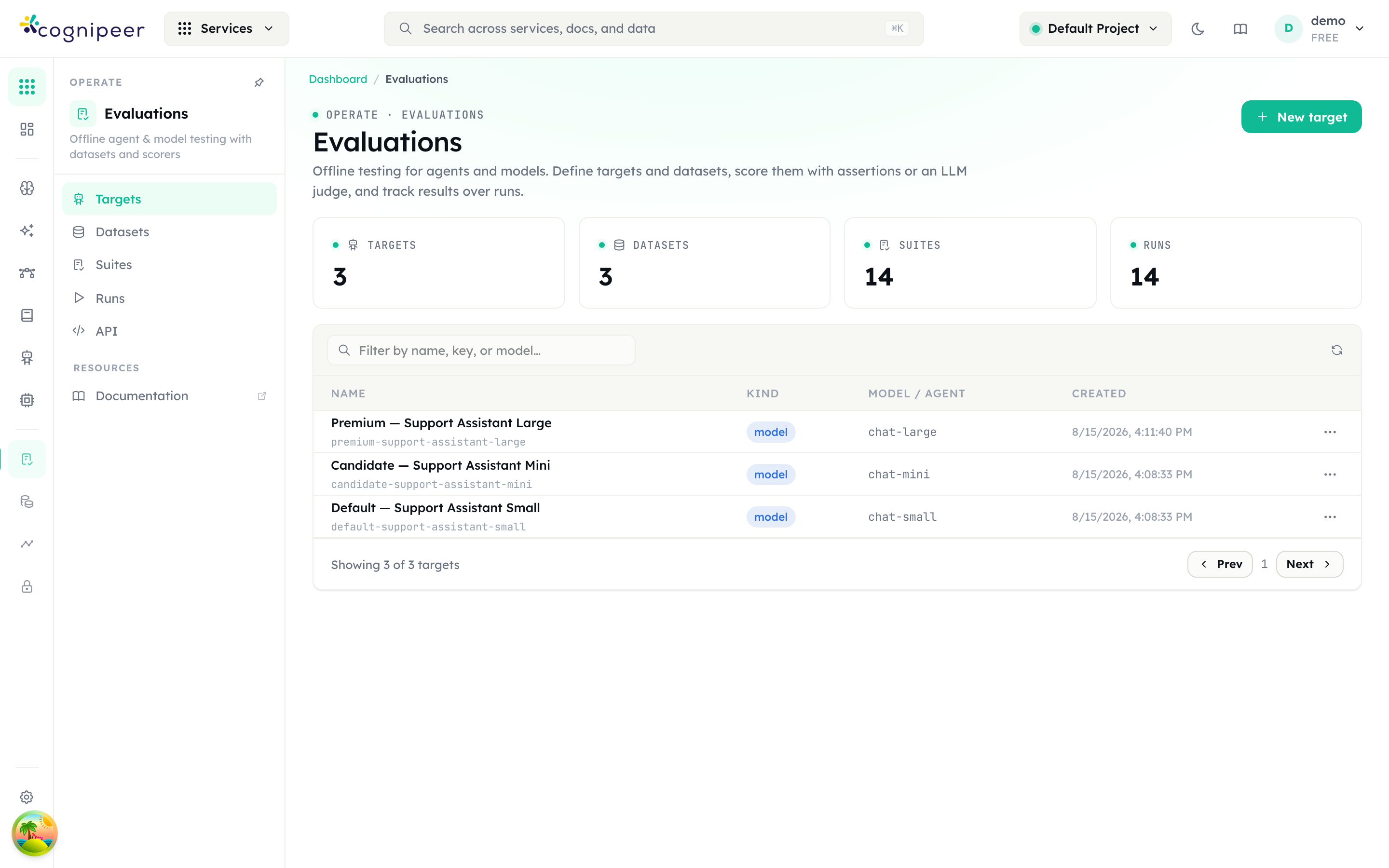
The demo comparison, graded on answer similarity against what the default model actually returned:
| Model | Pass rate | Avg score | Avg latency | Cost |
|---|---|---|---|---|
| Default (Small) — control | 0.602 | 0.601 | 427 ms | $0.0336 |
| Candidate (Mini) | 0.113 | 0.435 | 214 ms | $0.0060 |
| Premium (Large) | 0.102 | 0.488 | 1,466 ms | $0.3548 |
Mini is 82% cheaper and twice as fast. It is also wrong: of the 112 gradeable items, only 21 answers stayed close to what production returned. The cheap model changes roughly eight answers in ten.
This is the point of the whole exercise. The naive comparison — the one with the empty assertion scorer — said "identical quality, 82% cheaper" and would have shipped a regression to every customer. The measured comparison stopped it.
The rule: never switch a model on price alone. Switch on pass-rate parity at a lower cost, measured on your own traffic.
About these numbers
They come from a synthetic demo tenant whose upstream is a local stand-in, deliberately configured so the cheaper tier answers more tersely. They are not a claim about any real model. The method is what transfers — run it on your own traffic and your own candidates.
Note also that evaluation runs deliberately do not write usage or spend logs. Testing twenty models will not pollute your production cost reports; the per-run cost above is computed by the run itself.
Doing this at scale (Enterprise)
Everything above is community. If you have an Enterprise licence, three surfaces automate this loop:
| Surface | What it does |
|---|---|
| Recommendations | Reprices your observed traffic against candidate models and ranks the switches worth making. No model is called — it is a static what-if. |
| Parity tests | Replays a candidate against a snapshot dataset and scores it, so the token and quality deltas are measured rather than assumed. Started from a row action on Recommendations. |
| Model matrix | One dataset against many candidates in a single run, compared side by side on pass rate, judge score, tool fidelity and measured cost per item. |
The relationship between the first two is the interesting part: a what-if assumes the candidate uses the same token volume as the incumbent, because a static calculation cannot know otherwise. Once a parity test has actually measured the ratio for that pair, the recommendation is repriced from the measurement instead of the assumption. The estimate corrects itself as you test.
This is also why there is no "save tokens" objective to sort by: under a 1:1 assumption every candidate ties on tokens. Cost needs pricing, latency works from observed averages and needs none, and token savings cannot be estimated at all — only measured, which is what a parity test is for.
See Cost & Optimization for these screens in full.
Act 7 — Cut the tokens
Four levers, in descending order of payoff.
1. Shrink the tool menu
Tool definitions are re-sent on every model call. Most agents carry tools they rarely or never use.
Disable them per tool on the MCP server's Tools tab, and in the agent's tool selection. Then re-check Tool menu / call and Input tokens / AI call on the Analysis screen — the drop is immediate and measurable.
2. Trim the system prompt
Work the System prompt checks table top to bottom. Start with any fail. Moving one timestamp out of the prefix is worth more than any amount of word-trimming, because it restores prompt caching.
3. Kill repeated tool calls
The Repeated tool calls table gives you the tool, the exact arguments and the worst session. This is almost always a loop bug — the result is not being fed back — and fixing it removes both the tool latency and a model turn.
4. Cache and route
Enable semantic cache on the model for traffic with repeated questions, and split cheap from expensive work with a Dynamic LLM.
What the cache does to your charts
A semantic-cache hit logs empty usage. Cached traffic disappears from your token and spend charts except for the cache-hit counter, so your "savings" chart and your "traffic" chart will disagree. That is by design, but it surprises everyone the first time.
The cache is also inert for streaming requests, and entries are partitioned by a hash of the resolved model settings — changing a sampling parameter invalidates the whole cache for that model.
Act 8 — Prove it
Re-run the identical suite against the same dataset.
- Pass rate and average score versus your baseline run — did quality hold?
- Cost & Optimization → Reports over the same window — did spend actually fall?
A change that improves cost and holds pass rate is a result. A change that improves cost and drops pass rate is a decision, and it needs a person to make it — which is exactly why you measured.
Things that will bite you
| Pricing is not retroactive | Entering a price today does not price yesterday's traffic |
| Gateway logs carry no tool definitions | Gateway-sourced dataset items have no tool menu; only the tracing source can carry one |
| Tool-call turns have no reference answer | Grade them with the tool-call scorer, not a similarity scorer |
| An assertion scorer with no assertions passes | It reports 100% and measures nothing |
| Non-canonical event types | The timeline renders; every insight comes back empty |
| Semantic cache hits log no usage | Savings and traffic charts will disagree |
| A Dynamic LLM prices at zero | Cost is attributed to the child model, not the router |
Where to go next
- Build a dataset from production traffic — the snapshot and import wizards in full
- Route requests with a Dynamic LLM — splitting cheap from expensive
- Cost & Optimization — every screen in this guide, in reference form, including the Enterprise recommendation and parity surfaces
- Agent Tracing — the trace data model
- Evaluation & Analysis — scorers, suites and runs in detail
- Cost & Prescriptions API — driving all of this from a script